SWMM56

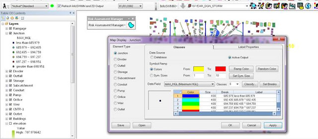
How to approximate the Flood polygon created in InfoSWMM RAM by using Arc Toolbox and Subcatchment Manager Tools Step 1 – Run InfoSWMM and use Map Display to show the Maximum HGL. This is just for reference to the later created polygons. Step 2 – not needed but as a check to Steps 3 to 5.  Use InfoSWMM RAM to show the area flooding based on the Maximum head or HGL.  This is an approximation of the flooding you would show with have with InfoSWMM 2D.  The maximum HGL is intersected with the DEM or TIN and the DEM elevations below the Maximum HGL are shown in Blue. Step 3 – Create a contour based on the Maximum HGL in the InfoSWMM run.  Use Contour in the InfoSWMM Browser to create the contour. Step 4 – The created Contour from the Maximum HGL Step 5 – Use the Polyline to Raster Arc Toolbox command to make a Raster from the Contour Step 6 – Optionally you an create a Raster using Convert in the InfoSWMM Subcatchment Manger. The tool creates a DEM from a Contour...

Graphing Infographic for InfoSWMM. Three different ways to run models : 1. Batch Mode 2. Single Run Manager 3. Changing Scenarios and then using the Single Run Manager 4. Your number one debugging tool is the System graphs, it tells you the total rainfall, runoff, flooding, outflow and storage in one easy to see graph or table

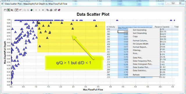
How to Use Scatter Plots in the DB Output tables of #InfoSWMM All of the SWMM5 output tables are available in the output report manager of InfoSWMM and H2OMap SWMM.  A key output table is the conduit summary table where the maximum link values are shown.  You can use the right mouse click to see the statistics, plot, frequency plot, histogram graph and scatter graph for the selected column.  If you select two columns you can make a scatter plot.  An interesting scatter graph is the d/D or capacity of the pipe versus q/Qfull for the pipe.  Qfull is based on the full pipe depth, area and hydraulic radius using the bed slope.  Due to the fact that InfoSWMM, SWMM5 and H2OMap SWMM use the full St. Venant solution you can have a q/Qfull greater than 1 when the d/D is less than 1.  Here are some St. Venant solution in SWMM5 blogs for reference. http://www.swmm5.net/search/label/St.%20Venant http://www.swmm5.net/2016/10/more-st-venant-equations-in-swmm5.h...

RDII Analyst, SWMM5 and ICM SE - Diagram of R, T and K parameters for RDII.  RDII Analyst in H2OMap SWMM and #InfoSWMM can export using the SWMM5 Export Exchange tool SWMM5 files with calibrated RTK parameters for #SWMM5 and #InfoWorks_ICM

How to Use Arc Map Selection to add to Domains in #InfoSewer and #InfoSWMM: Use the Arc Map Selection Tools Select a layer of Nodes or Links in Arc Map Add your elements to the Arc Map Selection and finally Add the selected elements from Arc Map to the InfoSewer Domain (Bullet 4) How to Use Arc Map Selection to add to Domains in #InfoSewer and #InfoSWMM

This blog shows the relationship between the terms dq1, dq2, dq3 and dq4 in the SWMM5 code and the St. Venant Partial Differential Equations. dq2 = Time Step * Area wtd * (Head Downstream – Head Upstream) / Link Length or dq2 = Time Step * Area wtd * (HGL) / Link Length Qnew = (Qold – dq2 + dq3 + dq4) / ( 1 + dq1) when the force main is full dq3 and dq4 are zero and Qnew = (Qold – dq2) / ( 1 + dq1) The dq4 term in dynamic.c uses the area upstream (a1) and area downstream (a2), the midpoint velocity, the sigma factor (a function of the link Froude number), the link length and the time step or dq4 = Time Step * Velocity * Velocity * (a2 – a1) / Link Length * Sigma the dq3 term in dynamic.c uses the current midpoint area (a function of the midpoint depth), the sigma factor and the midpoint velocity dq3 = 2 * Velocity * ( Amid(current iteration) – Amid (last time step) * Sigma dq1 = Time Step * RoughFactor / Rwtd^1.333 * |Velocity| The weighted area (Awtd) is used in the dq2 term of the St...

In this blog we example the Froude Number values computed in SWMM5 as equations, table, graphs and units. We use a QA/QC version of SWMM 5 that lists many more link, node, system and Subcatchment variables than the default SWMM 5 GUI and engine. This blog also applies to #InfoSWMM and any software the uses the #SWMM5 engine.  SWMM 5 computes only one flow in the middle of the link but it uses depth, head, cross sectional area and hydraulic radius at the upstream, midpoint and downstream points of the link (Figure 1).  The Froude # is computed at all three points and if you could see the Froude # you will see a jump at times in a single link (Figure 2). Figure 1.  Computational points in #SWMM5 Figure 2.  Three locations of the Froude Number - it is possible to see where the Hydraulic Jump occurs in the link.

Overview In this blog we show how the St Venant terms are used in SWMM5 as equations, table, graphs and units. We use a QA/QC version of SWMM 5 that lists many more link, node, system and Subcatchment variables than the default SWMM 5 GUI and engine. This also applies to #InfoSWMM and any software the uses the #SWMM5 engine. SWMM5 is using is the most advanced equations as it takes into consideration the full dynamic (St. Venant) equations and not the more simplified kinematic wave / manning equations. The manning equation only considers the uniform flow conditions which represents a situation where the gravitational force on a column of water (due to the channel slope) balances out the frictional force. The full dynamic equations contains additional factors that affect the movement of water in a conduit or channel. These include the pressure force due to variation of depth along the length of the channel and the inertial (or convective acceleration) effect due to variation of flow ar...

Arc GIS Tools for 2D Polygon Processing Clip – restrict data to area of extents Buffer – offset polygon data Dissolve – merge polygons Multipart to Singlepart – make features individual (need to run after using dissolve) Repair geometry – fix bad geometry Erase – remove features inside areas Integrate – align polygons

Step 0 is to define the domain and use the Custom tool in Tools, Step 1 is to define the data source Step 2 is to define the fields to show in the table Step 3 is to define the source (click on Domain) and Step 4 is to view the output table.

New Modified Rational Formula in InfoSWMM InfoSWMM H2OMap SWMM now offers 12 choices for modeling surface runoff including the new Modified Rational Method (MRM) 1. EPA SWMM 5 Nonlinear Reservoir 2. The Colorado Urban Hydrograph Procedure (CUHP) 3. NRCS (SCS) Dimensionless Unit Hydrograph Method 4. NRCS (SCS) Triangular Unit Hydrograph Method 5. Delmarva Unit Hydrograph 6. Snyder Unit Hydrograph Method 7. Clark Unit Hydrograph Method 8. Espey Unit Hydrograph Method 9. Santa Barbara Urban Hydrograph Method 10. San Diego Modified Rational Method 11. Modified Rational Method  (NEW!) 12.  German Runoff (NEW!) The Rational method is a widely used technique for estimation of peak flows from urban and rural drainage basins (Maidment 1993; Mays 2001). Stormwater modeling applications such as the design of detention basins require knowledge of total inflow volume obtained from runoff hydrographs. For these applications peak flow information alone may not be sufficient.  The San Di...

How to Use Non-Steady Periods in  InfoSWMM How to Use Non-Steady Periods in  InfoSWMM

A Hot Start File in InfoSWMM  or SWMM 5 is important as it provides initial   depths, initial flows and  initial settings for the hydrology and hydraulics features of the SWMM 5 engine.    You  have three options: Save a hot Start File at the  end of the  simulation, Use a hot Start File  at the beginning of  the simulation, Create a hot start file  from  the a  time during  the  Map Display If you change any of the network  types or add new links and nodes then  the Hot Start file needes to be recreated.  InfoSWMM use the Tab File in  the Run Manager to name the Hot Start File (Figure 1).   Each and  every Scenario in InfoSWMM  can  use or Save a different scenario with different starting  and ending  times  (Figure 2).  If you USE  a Hot  Start  File then: The  new  simulation  starts at the end  of  the  ol...

InfoSWMM Sustain Generation V2.0 Delivers Significant Advancements for Comprehensive Urban Stormwater Treatment and Analysis Latest Release Confirms Product’s Role as Industry Leading GIS-Centric Solution for Determining Optimal Green Infrastructure Strategies Broomfield, Colorado, USA, April 12, 2016 Innovyze, a leading global innovator of business analytics software and technologies for smart wet infrastructure, today announced  worldwide availability of the V2.0 Generation of its industry-leading  InfoSWMM Sustain  for comprehensive urban stormwater treatment and analysis. The new version lets users quickly and reliably determine optimal green infrastructure strategies for reducing volume and peak flows to combined sewer systems as well as evaluating the benefits of distributed green infrastructure implementation on water quantity and quality in urban streams. InfoSWMM Sustain  is a comprehensive geocentric decision support system created to assist stormwater mana...

Innovyze Further Expands RDII Analyst Functionality, Setting New Standard for Sanitary and Combined Sewer System Model Calibration New Features Allow Unprecedented Analysis and Comparison of Rainfall-Derived Inflow and Infiltration Data, Parameters for Complex Sewers Broomfield, Colorado, USA, February 23, 2016 Innovyze, a leading global innovator of business analytics software and technologies for smart wet infrastructure, today announced the newest release of its  RDII Analyst  (Rainfall-Derived Inflow and Infiltration) for  InfoSWMM  and  H 2 OMAP SWMM . The new version delivers expanded functionality, incorporating many advanced Genetic Algorithm (GA) optimization features. It increases its unmatched productivity by openly inviting the users to further adjust the dry weather flow (DWF) and RTK parameters (with initial and maximum monthly storages for continuous simulation) to achieve a better fit and ultimately a better model based on their experiences. The ...

One of the most powerful InfoSWMM and H2OMAP SWMM Application Tools from Innovyze is RDII Analyst.  RDII Analyst will separate out the Groundwater base flow, Dry Weather Flow (DWF), DWF Patterns, estimate the Wet Weather flow component or RDII  Rainfall -Derived Infiltration Inflow (I&I) and use a Genetic Algorithm to find  the best fit 12 RTK parameters for RDII modeling.  This powerful tool can  be used for RTK flow in InfoSWMM, H2OMAP SWMM, InfoSewer, SWMM 5 and InfoWorks ICM.  Figure 1 shows one of the  end results of RDII Analyst – a correlation plot of Observed versus Calibrated RDII Volume for the simulated events. RDII Analyst is a significant improvement over the EPA SSOAP program, performs QA/QC of rainfall and flow monitoring data and decomposes the flow data into Dry-Weather Flow (DWF) and Wet-Weather Flow (RDII) components using criteria such as rainfall threshold. The DWF component is further analyzed to construct a DWF pattern t...