SWMM56

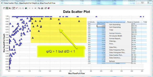
How to Use Scatter Plots in the DB Output tables of #InfoSWMM All of the SWMM5 output tables are available in the output report manager of InfoSWMM and H2OMap SWMM.  A key output table is the conduit summary table where the maximum link values are shown.  You can use the right mouse click to see the statistics, plot, frequency plot, histogram graph and scatter graph for the selected column.  If you select two columns you can make a scatter plot.  An interesting scatter graph is the d/D or capacity of the pipe versus q/Qfull for the pipe.  Qfull is based on the full pipe depth, area and hydraulic radius using the bed slope.  Due to the fact that InfoSWMM, SWMM5 and H2OMap SWMM use the full St. Venant solution you can have a q/Qfull greater than 1 when the d/D is less than 1.  Here are some St. Venant solution in SWMM5 blogs for reference. http://www.swmm5.net/search/label/St.%20Venant http://www.swmm5.net/2016/10/more-st-venant-equations-in-swmm5.h...

This blog shows the relationship between the terms dq1, dq2, dq3 and dq4 in the SWMM5 code and the St. Venant Partial Differential Equations. dq2 = Time Step * Area wtd * (Head Downstream – Head Upstream) / Link Length or dq2 = Time Step * Area wtd * (HGL) / Link Length Qnew = (Qold – dq2 + dq3 + dq4) / ( 1 + dq1) when the force main is full dq3 and dq4 are zero and Qnew = (Qold – dq2) / ( 1 + dq1) The dq4 term in dynamic.c uses the area upstream (a1) and area downstream (a2), the midpoint velocity, the sigma factor (a function of the link Froude number), the link length and the time step or dq4 = Time Step * Velocity * Velocity * (a2 – a1) / Link Length * Sigma the dq3 term in dynamic.c uses the current midpoint area (a function of the midpoint depth), the sigma factor and the midpoint velocity dq3 = 2 * Velocity * ( Amid(current iteration) – Amid (last time step) * Sigma dq1 = Time Step * RoughFactor / Rwtd^1.333 * |Velocity| The weighted area (Awtd) is used in the dq2 term of the St...

Overview In this blog we show how the St Venant terms are used in SWMM5 as equations, table, graphs and units. We use a QA/QC version of SWMM 5 that lists many more link, node, system and Subcatchment variables than the default SWMM 5 GUI and engine. This also applies to #InfoSWMM and any software the uses the #SWMM5 engine. SWMM5 is using is the most advanced equations as it takes into consideration the full dynamic (St. Venant) equations and not the more simplified kinematic wave / manning equations. The manning equation only considers the uniform flow conditions which represents a situation where the gravitational force on a column of water (due to the channel slope) balances out the frictional force. The full dynamic equations contains additional factors that affect the movement of water in a conduit or channel. These include the pressure force due to variation of depth along the length of the channel and the inertial (or convective acceleration) effect due to variation of flow ar...

Subject:    Lambda Calculus and Link Variables in the InfoSWMM, H2OMAP SWMM and SWMM 5 Dynamic Wave Solution Successive under-relaxation for the SWMM 5 Dynamic Wave Solution by  dickinsonre Subject:   Successive under-relaxation for the SWMM 5 Dynamic Wave Solution SWMM 5 uses the method of Successive under-relaxation to solve the  Node Continuity Equation  and the  Link Momentum/Continuity Equation  for a time step.  The dynamic wave solution in dynwave.c will use up to 8 iterations to reach convergence before moving onto the next time step.  The differences between the link flows and node depths are typically small (in a non pumping system) and normally converge within a few iterations unless you are using too large a time step.  The number of iterations is a minimum of two with the 1 st  iteration NOT using the under-relaxation parameter omega. The solution method can be term successive approximation, fixed iteration or...

Subject:   How is the St Venant Equation Solved for in the Dynamic Wave Solution of SWMM 5? How is the St Venant Equation Solved for in the Dynamic Wave Solution of SWMM 5? by  dickinsonre Subject:    How is the St Venant Equation Solved  for in the Dynamic Wave Solution of S WMM 5? An explanation of the four St. Venant Terms in SWMM 5 and how they change for Gravity Mains and Force Mains. The HGL is the water surface elevation in the upstream and downstream nodes of the link. The HGL for a full link goes from the pipe crown elevation up to the rim elevation of the node + the surcharge depth of the node.  The four terms are: dq2  = Time Step * Awtd * (Head Downstream – Head Upstream) / Link Length or dq2  = Time Step * Awtd * ( HGL ) / Link Length Qnew  = (Qold – dq2 + dq3 + dq4) / ( 1 + dq1) when the force main is full dq3 and dq4 are zero and Qnew...

Force Main Friction Loss in InfoSWMM and the Transition from Partial to Full Flow by  dickinsonre Subject:   Force Main Friction Loss in InfoSWMM and the Transition from Partial to Full Flow You can model Force Main friction loss in InfoSWMM using either Darcy Weisbach or Hazen Williams as the full pipe friction loss method (see Figure 1 for the internal definition of full flow).   A  function called ForceMain in InfoSWMM whose purpose is to compute the Darcy-Weisbach friction factor for a force main using the  Swamee and Jain approximation to the Colebrook-White equation  .   No matter which method you use for full flow the  program will use Manning's equation to calculate the loss in the link when the link is not full (see Figure 2 for the equations used for calculating the friction loss – variable dq1 in the St Venant equation for InfoSWMM).    The regions for the different friction loss equations are shown in Figu...

Subject:   An Example of the Importance of the Term DQ4 in the SWMM 5 St Venant Solution An Example of the Importance of the Term DQ4 in the SWMM 5 St Venant Solution by  dickinsonre Subject:    An Example of the Importance of the Term DQ4 in the SWMM 5 St Venant Solution The four terms are are used in the new flow for a time step of Qnew: Qnew  = (Qold – dq2 + dq3 + dq4) / ( 1 + dq1) when the force main or gravity main is full dq3 and dq4 are zero and   Qnew  = (Qold – dq2) / ( 1 + dq1) The  dq4  term in dynamic.c uses the area upstream ( a1 ) and area downstream ( a2 ), the midpoint velocity, the sigma factor (a function of the link Froude number), the link length and the time step or dq4  = Time Step * Velocity * Velocity * (a2 – a1) / Link Length * Sigma where Sigma is a function of the Froude Number and the Keep, Dampen and Ignore Inertial Term Options.  Keep sets Sigma to 1 always and Dampen set Sigma based...

Note:   The Keep and Dampen options and their effect on the four main terms of the St Venant equation.  The Keep and Dampen options and their effect on the four main terms of the St Venant equation in SWMM5 by  dickinsonre Note:   The Keep and Dampen opt ions and their effect on the four main terms of the St Venant equation.  The four terms are are used in the new flow for a time step of Qnew: Qnew  = (Qold – dq2 + dq3 + dq4) / ( 1 + dq1) when the force main or gravity main is full dq3 and dq4 are zero and   Qnew  = (Qold – dq2) / ( 1 + dq1) The  dq4  term in dynamic.c uses the area upstream ( a1 ) and area downstream ( a2 ), the midpoint velocity, the sigma factor (a function of the link Froude number), the link length and the time step or dq4  = Time Step * Velocity * Velocity * (a2 – a1) / Link Length * Sig...

Subject:    Surcharged Node and the Link Connection in SWMM 5 Surcharged Node and the Link Connection in SWMM 5 by  dickinsonre Subject:    Surcharged Node and the Link Connection in SWMM 5   A  surcharged   node  in  SWMM   5   uses this point iteration equation (Figure 1):   dY/dt = dQ / The sum of the Connecting Link values of  dQ/dH   where Y is the depth in the node, dt is the time step, H is the head across the link (downstream – upstream), dQ is the net inflow into the node and dQ/dHis the derivative with respect to H of the link  St Venant equation.   If you are trying to calibrate the surcharged node depth, the main calibration variables are the time step and the link  roughness:   1.    Mannings's...

Note:   How to Search These Blogs for Information How to Search These Blogs for Information about SWMM5, InfoSWMM or InfoSewer by  dickinsonre Note:   How to  Search   These   Blogs  for  Info rmation   In each of the  blogs   search   for a term or a set of terms using the  search  button.   For example, here is  http://swmm5.blogspot.com   with a  search  for venant     An equivalent  Search  in  http:// www.swmm2000.com     An equivalent  Search  in  http:// swmm5.wordpress.com/     via Blogger   http://www.swmm5.net/2013/08/ how-to-search-these-blogs-for. html dickinsonre  |  August 4, 2013 at 7:28 am  | Tags:  Blogger ,  H2oMAP SWMM ,  IFTTT ,  InfoSWMM , swmm5  | Categories:  H2OMAP SWMM ,  InfoSWMM ,  swmm5  | URL:  http://wp.me/...

Subject:    SWMM 5 Loss Term Values for various velocities and K values SWMM 5 has three loss terms available for each link:  Entrance, Exit and Other losses.  The Entrance loss uses the upstream link velocity, the  Other loss uses the center link velocity and the Exit loss uses the downstream link velocity.  The general form of the loss term in the St. Venant equation is K*V^2/2g Table 1 shows the loss in feet of head for various combinations of velocity and K value.  If you want to  simulate a little loss of head at each node then a small value of K should be used otherwise the cumulative loss in the whole networks will be many feet of head.   Loss Term units equals K * V^2/2g = ft/sec * ft/sec * sec^2/ft = ft Table 1:  Loss in feet of head for various combinations of velocity and K values. Velocity (ft/sec) K K K K K K 0.050 0.100 0.250 0.500 0.750 1.000 1 0.001 0.002 0.004 0.008 0.012 0.016 2 0.003 0.006 0.016 0.031 0.047 0.062 3...